Quickstart#

Example#

Here we proivde a simple example and more explanation be in the following sections.

import pandas as pd
from modrover.api import Rover

# sample data
data = pd.DataFrame({
    "obs": [1.0, 2.0, 3.0, 4.0, 5.0],
    "cov0": [1.1, 2.1, 2.8, 3.6, 5.2],
    "cov1": [6.1, 2.2, 1.6, 5.8, 0.5],
    "holdout0": [0, 0, 0, 0, 1],
    "holdout1": [1, 0, 0, 0, 0],
})

# create rover object
rover = Rover(
    model_type="gaussian",
    obs="obs",
    cov_fixed=["intercept"],
    cov_exploring=["cov0", "cov1"],
    holdouts=["holdout0", "holdout1"],
)

# fit and predict
rover.fit(data=data, strategies=["full"], top_pct_learner=0.5)
pred = rover.predict(data)

# plot the spread of the coefficients
fig = rover.plot()

# learner information and the summary of the ensemble information
learner_info = rover.learner_info
summary = rover.summary

Data#

ModRover works with data in the form of the Pandas data frames. In the dataset, we need to provide the observations, covariates of interest, other important information, e.g. the weight of the data point and the holdout columns for computing the out-of-sample performance.

Rover#

Rover is the main class that user need to interact with. Here we provide description of the arguments in the example. For more details please check the API Reference.

model_type corresponding to the model family, currently we provide classical choices {"gaussian", "poisson", "binomial"}
obs is the column name in the dataset corresponding to the observations
cov_fixed is the list of column names corresponding to the covariates user want to include in all of the learners. The most common choice is ["intercept"], which indicate every learner will have the intercept as part of its covariates. (User don’t have to create "intercept" in their dataset, it will be automatically generated)
cov_exploring is the list of column names corresponding to the covariates user want to test the inclusion.
holdouts is the list of column names corresponding to the indicators of holdout. The column should contain only 0 or 1, where 0 marks the row as the training data and 1 for testing data. This set of columns will be used to divide the training and testing data and evaluate the out-of-sample performance.

Rover.fit#

After creating the rover instance, we can call fit function to fit all the base learners and ensemble the super learner. For more details please check API Reference.

data is the dataframe that contains all necessary columns defined in the rover object previously
strategies is a list of strings corresponding to the strategies we want to use to explore the model space. Currently the strategy provide are {"full", "forward", "backward"}, where "full" will fit every possible covariate-combinations in cov_exploring. In this example since we only have two covariates, there are only four possibilities, we can afford to fit all combinations. Usually when we have lots of covariates "forward" and "backward" are more suitable options. "forward" strategy starting with the model only include the covariates in cov_fixed and add one covariate at a time depending on the model performance. And "backward" strategy start with the model include all covariates in cov_fixed and cov_exploring and remove one covirate at a time depending on the model performance. These two strategies allow us to explore the model space more efficiently rather than go through every poissible combination.
top_pct_learner is an ensemble option. In this example, we will only include the top 50% of the fitted models according to their score to ensemble the super learner. The other two ensemble options are, top_pct_score and coef_bounds.

After fitting the model, we will be able to access the super learner. To get the estimated coefficients and the variance-covariance matrix,

>>> rover.super_learner.coef
array([0.02527973, 1.00497306, 0.        ])
>>> rover.super_learner.vcov
array([[ 0.0306691 , -0.01050203,  0.        ],
       [-0.01050203,  0.00474495,  0.        ],
       [ 0.        ,  0.        ,  0.        ]])

Rover.predict#

Rover.predict is used to generate predictions. User need to make sure to include all covariate columns. If we specify the arguments as in the example, the function will return a single array as the prediction. If we also want the uncertainty interval, we need to set return_ui=True. By default it will return the point prediction and the 95% uncertainty interval, if we want 90% uncertainty interval, we can specify alpha=0.1.

>>> rover.predict(data)
array([1.1307501 , 2.13572317, 2.83920431, 3.64318276, 5.25113966])
>>> rover.predict(data, return_ui=True)
array([[1.1307501 , 2.13572317, 2.83920431, 3.64318276, 5.25113966],
       [0.90466489, 1.966146  , 2.65266606, 3.39104678, 4.81396876],
       [1.35683532, 2.30530033, 3.02574256, 3.89531874, 5.68831056]])

Rover.plot#

Rover.plot create a diagnostic plot of the spread of the coefficients across different learners. It gives us a general sense of how sensitive the covariate coefficients are depending on the covariates we include in the model.

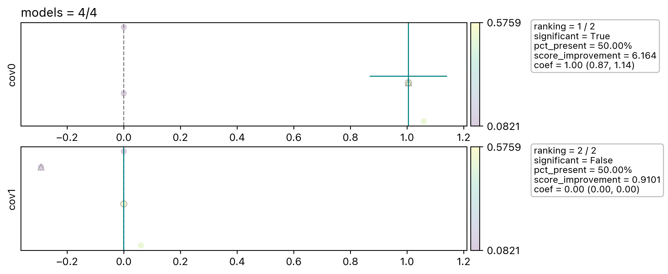
Each row panel corresponding to one covariate in cov_exploring. In this example we will only see four dots in each panel. We only have two covariates and it produces in-total four base learners. The points are arrange horizontally by their coefficients value and vertically by random value. The triangle marker marks the model only include cov_fixed and the corresponding covariate. The circle marker marks the final learners included in the ensemble. The vertical and horizontal teal line mark the ensembled coefficents and their uncertainty. And there are more information plotted in the text box.

Diagnostics#

At last, rover also provide two diagnostic data frame to help user track the status and results.

Learner Info#

rover.learner_info contains all the status of all the learners and if they are valid to be included in the final ensemble.

learner_id	status	mu_intercept	mu_cov0	mu_cov1	score	coef_valid	valid	weight
()	ModelStatus.SUCCESS	3.0	0.0	0.0	0.0820849986238988	True	True	0.0
(0,)	ModelStatus.SUCCESS	0.025279734769995375	1.0049730625777042	0.0	0.5758624583075163	True	True	1.0
(1,)	ModelStatus.SUCCESS	3.946640012302013	0.0	-0.29217284330309057	0.09334432412858795	True	True	0.0
(0, 1)	ModelStatus.SUCCESS	-0.331985590803968	1.059348804954034	0.06059047164815646	0.5054786621816283	True	True	0.0

Here learner_id encode the covariates configuration. In this example, (,) corresponding to the model only includs intercept, (0,) is for intercept + cov0 and (0, 1) is for intercept + cov0 + cov1.

Summary#

rover.summary contains covariates information of the final ensemble.

cov	coef	coef_sd	pct_present	single_score	present_score	not_present_score	score_improvement	ranking	coef_lwr	coef_upr	significant
cov0	1.0049730625777042	0.06888362821620424	0.5	0.5758624583075163	0.5406705602445723	0.08771466137624337	6.163970216169671	1	0.8699611512739439	1.1399849738814645	True
cov1	0.0	0.0	0.5	0.09334432412858795	0.2994114931551081	0.32897372846570755	0.9101380057049723	2	0.0	0.0	False